Introduction
In this blog post, I want to show how you can get a first impression on how you can cut a monolithic application into separated components that make sense from a business’ perspective. This method can help you to identify meaningful Bounded Contexts (source code that has a high conceptual cohesion in means of business terminology) for your application that should follow a Domain-Driven Design.
We achieve this with a nice D3 chord visualization (created by Pasha, licensed under GPL 3.0) combined with jQAssistant / Neo4j graph analysis. jQAssistant can scan your Java application and store a graph of your software in a Neo4j graph database. This graph can then be enriched with Cypher to get additional nodes and relationships as well as queried as you need it – for your specific use cases.
To quickly get started, there is already a nice showcase project on GitHub that we can use to start immediately – the “jQAssistanterized” version of Spring PetClinic. Just clone this repository and build it with the Maven command mvn clean install -DskipTests. I also wrote about how one can build a higher level view of the source code as well as analyzing dependencies between Java source code.
It’s time to combine both approaches!
Marking components in code
In this section, we want to find out components in our application that would probably be suited for Bounded Contexts. The Spring PetClinic project already comes with some user-defined queries for subdomains (the “concept” business:Subdomain that’s defined in the self-validating, living architecture documentation) that are derived from naming conventions of some Java types. That means that there is already a relationship between source code and the business’ concepts existing – this will fit for our purpose.
We can query that graph directly via Python and py2neo to get the data in a JSON format from Neo4j. For effectiveness reasons (and a nice inline, tabular visualization as well), we wrap that result in a Pandas DataFrame for further processing.
import py2neo
import pandas as pd

graph = py2neo.Graph()
subdomains_query="""
MATCH (t:Type)-[:BELONGS_TO]->(s:Subdomain)
RETURN s.name as Name, COUNT(t) as Types
"""
result = graph.run(subdomains_query).data()
df = pd.DataFrame(result)
df.head()
For our analysis, we additionally need to mark all Java types that don’t belong to an existing business subdomain. To keep it simple, we just add a new Subdomain node with the name “Framework” to the graph and connect all the remaining types without a connection to an existing Subdomain node.
framework_query="""
CREATE (s:Subdomain { name: "Framework" })
WITH s
    MATCH (:Project)-[:CONTAINS*]->(t:Type)
    WHERE NOT (t)-[:BELONGS_TO]->(:Subdomain)
    MERGE (t)-[:BELONGS_TO]->(s)
RETURN s.name as Name, COUNT(t) as Types
"""
result = graph.run(framework_query).data()
df = pd.DataFrame(result)
df.head()
That’s all what it takes now for marking software elements and their relationships to business subdomains aka Bounded Countexts.
Dependencies between Subdomains
Here comes the actual analysis part: We search all dependencies (with the :DEPENDS_ON relationship) between Types and retrieve the Subdomain node / information for each of them.
The Cypher query for Neo4j is straightforward:
query="""
MATCH
    (s1:Subdomain)<-[:BELONGS_TO]-
    (type:Type)-[r:DEPENDS_ON*0..1]->
    (dependency:Type)-[:BELONGS_TO]->(s2:Subdomain)
RETURN s1.name as from, s2.name as to, COUNT(r) as x_number
"""
result = graph.run(query).data()
df = pd.DataFrame(result)
df.head()
This query returns all Subdomains with the number of relationships between all the types of the same Subdomain as well as other Subdomains.
For example, from the “Visit” subdomain, there is one relationship (x_number, the “x” is just there for the right ordering of the DataFrame columns) to the “Framework” subdomain.
Because subdomain can be seen as Bounded Contexts, we get a nice overview between existing dependencies between them.
Export data for visualization
The interactive chord visualization needs the result in the JSON format as list of dictionary entries in the format “from, to, number”. So we export it accordingly.
import json
json_data = df.to_dict(orient='split')['data']
with open ( "vis/chord_data.json", mode='w') as json_file:
    json_file.write(json.dumps(json_data, indent=3))
json_data[:5]
Interactive Analysis
After this, we can open the HTML page where D3 does it’s magic.
In a chord diagram, the data / subdomains are ordered around a circle. The numbers in the parenthesis are the number of inter-relationships between data / types.
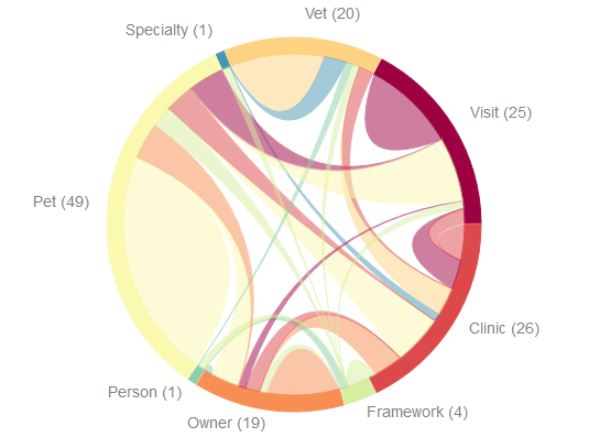
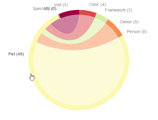
When hovering over a subdomain’s text or the corresponding arc, the chord diagram will show you all dependencies that go from this subdomain to other subdomains (different color than the current subdomain) and the dependencies that refer to types in the same subdomain (same color). This can show you which subdomains already are on a high degree self-contained. this information can guide you for first separations of your application into Bounded Contexts.
Additionally, the number of dependencies into the other subdomains is updated as well.
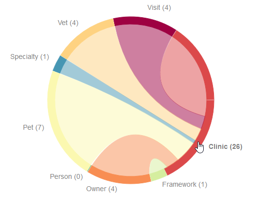
With this, we can identify subdomains where it could be hard to create a Bounded Context from. For example, the Clinic subdomain has dependencies in almost all other subdomains. Looking into the code, we can see that the Clinic subdomain is kind of orchestration layer or facade for the accessing all other subdomains. This is an important information because we have to treat this component different than others.
Summary
Thanks to jQAssistant and Neo4j, the necessary data for this visualization is easy to retrieve. The interactive chord diagram comes quite useful if you want to cut some intertwined components into separate ones e. g. for creating microservices (there, finally I said it!).
But in huge systems, this could be very cumbersome. We could do that also more on an analytical basis based on the data. But this is a topic for another blog post 🙂
This blog post is also avaiable as interactive notebook on GitHub.
Pingback:Community Blog Posts · jQAssistant
Do you know ColorBrewer http://colorbrewer2.org/#type=sequential&scheme=BuGn&n=3?
It’s terrific for generating legible color schemes
No, but I can brew colors with matplotlib and D3. I was just too lazy to do it for this visualization 🙂
Pingback:This Week in Neo4j – 28 October 2017 – Cloud Data Architect
Pingback:My talk at JAX 2018 – feststelltaste
why you also wrote about how one can build a higher level view of the source code?