TL;DR I show how I determine the parts of an application that trigger unnecessary SQL statements by using graph analysis of a call tree.
Introduction
General claim
We don’t need more tools that show use more problems in our software. We need ways to determine the right problem to solve. But often we just fix the symptoms on the surface rather than the underlying problems. I find that approach non-professional and want to do my part to improve this situation by delivering root cause analysis of symptoms to get to the real problems in our software.
What you will see
In this notebook, I’ll show you one of my approaches for mining performance problems based on application runtime performance analysis. In general, I use this approach to make the point that there are severe design errors that have a negative influence on the application’s overall performance. In this example, I show you how I determine the reasons behind a massive amount of executed SQL statements in an application step by step.
The key idea is to use graph analysis to analyze call stacks that were created by a profiling tool. With this approach, I’m not only able to show the hotspots that are involved in the performance issue (that show that some SQL statements take long to execute or are executed too often), but also the reasons behind these hotspots. I achieve this by extracting various additional information like the web requests, application’s entry points and the triggers within the application causing the hotspots.
This is very helpful to determine the most critical parts in the application and gives you a hint where you could start improving immediately. I use this analysis at work to determine the biggest performance bottleneck in a medium sized application (~700 kLOCs). Based on the results, we work out possible improvements for that specific hotspot, create a prototypical fix for it, measure the fix’s impact and, if the results are convincing, roll out the fix for that problem application wide (and work on the next performance bottleneck and so on).
I hope you’ll see that this is a very reasonable approach albeit the simplified use case that I show in this blog post/notebook.
Used software
Before we start, I want to briefly introduce you to the setup that I use for this analysis:
- Fork of the Spring sample project PetClinic as application to torture
- Tomcat 8 installation as servlet container for the application (standalone, for easier integration of the profiling tool)
- JMeter load testing tool for executing some requests
- JProfiler profiler for recording performance measures
- jQAssistant static analysis tool for reading in call trees
- Neo4j graph database and Cypher graph query language for executing the graph analysis
- Pandas, py2neo and Bokeh on Jupyter* as documentation, execution and analysis environment
The first ones are dependent on the environment and programming language you use. jQAssistant, Neo4j and Pandas are my default environment for software analytics so far. I’ll show you how all those tools fit together.
So let’s get started!
*actually, what you see here, is the result of an executed Jupyter notebook, too. You can find that notebook on GitHub.
Performance Profiling
As a prerequisite for this analysis, we need performance profiling data gathered by a profiler. A profiler will be integrated into the runtime environment (e. g. Java Virtual Machine) of your application and measures diverse properties like method execution time, number of web service calls, executed SQL statements etc. Additionally, we need something that uses or clicks through our application to get some numbers. In my case, I run the Spring PetClinic performance test using JMeter.
As profiling tool, I use JProfiler to record some performance measures while the test was running.
<advertisment>
At this point, I want to thank ej-technologies for providing me with a [free open-source license](https://www.ej-technologies.com/buy/jprofiler/openSource) for JProfiler that enables this blog post in exchange of mentioning their product:

JProfiler is a great commercial tool for profiling Java application and costs around 400 €. It really worth the money because it gives you deep insights how your application performs under the hood.
</advertisment>
Also outside the advertisement block, I personally like JProfiler a lot because it does what it does very very good. Back to the article.
The recording of the measures starts before the execution of the performance test and stops after the test has finished successfully. The result is stored in a file as so-called “snapshot” (the use of a snapshot enables you to repeat your analysis over and over again with exactly the same performance measures).
What we usually need for performance analysis is a recorded runtime stack of all method calls as a call tree. A call tree shows you a tree of the called methods. Below, you can see the call tree for the called methods with their measured CPU wall clock time (aka the real time that is spent in that method) and the number of invocations for a complete test run:
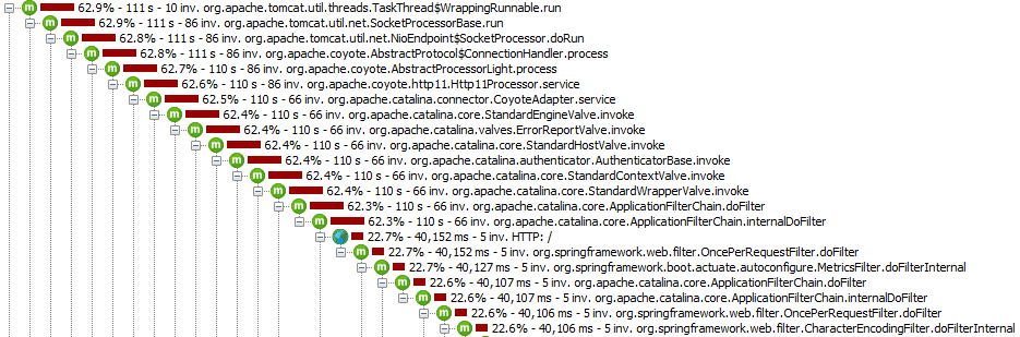
With such a view, you see which parts of your application call which classes and methods by drilling down the hierarchy by hand:
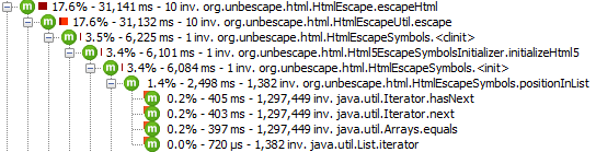
But there is more: You can also “turn around” the call tree and list all the so-called “HotSpots”. Technically, e. g. for CPU HotSpots, JProfiler sums up all the measurements for the method call leafs that take longer than 0.1% of all method calls. With this view, you see the application’s hotspots immediately:
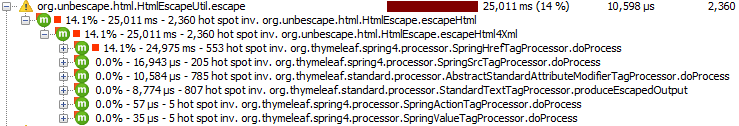
These views are also available for other measures like web service calls, file accesses or DB calls, that is shown below:
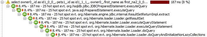
This is the data that we need for our SQL statement analysis. The big problem is, that we can’t easily see where all those SQL statements come from because we just see the isolated SQL statements.
And this is where our journey begins…
Reading XML into Neo4j
The input data
For further processing, we export such a call tree into a XML file (via the JProfiler GUI or the command line tool jpexport). If we export the data of the SQL hotspots (incl. the complete call tree) with JProfiler, we’ll get a XML file like the following:
with open (r'input/spring-petclinic/JDBC_Probe_Hot_Spots_jmeter_test.xml') as log:
    [print(line[:97] + "...") for line in log.readlines()[:10]]
For a full version of this file, see GitHub: https://github.com/feststelltaste/software-analytics/blob/master/notebooks/input/spring-petclinic/JDBC_Probe_Hot_Spots_jmeter_test.xml
This file consists of all the information that we’ve seen in the JProfiler GUI, but as XML elements and attributes. And here comes the great part: The content itself is graph-like because the XML elements are nested! So the <tree> element contains the <hotspot> elements that contain the <node> elements and so on. A case for a graph database like Neo4j!
But how do we get that XML file into our Neo4j database? jQAssistant to the rescue!
Scanning with jQAssistant
jQAssistant is a great and versatile tool for scanning various graph-like structured data into Neo4j (see my experiences with jQAssistant so far for more information). I just downloaded the version 1.1.3, added the binary to my PATH system variable and executed the following command (works for jQAssistant versions prior to 1.2.0, I haven’t figured it out how to do it with newer versions yet):
jqassistant scan -f xml:document::JDBC_Probe_Hot_Spots_jmeter_test.xml
This will import the XML structure as a graph into the Neo4j graph database that is used by jQAssistant under the hood.
Exploring the data
So, if we want to have a quick look at the stored data, we can start jQAssistant’s Neo4j embedded instance via
jqassistant server
open http://localhost:7474, click in the overview menu at the label File, click on some nodes and you will see something like this:
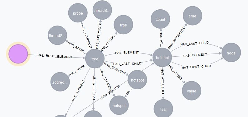
It shows the content of the XML file from above as a graph in Neo4j:
- The pink node is the entry point – the XML file.
- To the right, there is the first XML element <tree> in that file, connected by the HAS_ROOT_ELEMENT relationship.
- The <tree> element has some attributes, connected by HAS_ATTRIBUTE.
- From the <tree> element, there are multiple outgoing relationships with various <hotspot> nodes, containing some information about the executed SQLs in the referenced attributes.
- The attributes that are connected to these elements contain the values that we need for our purpose later on.
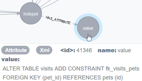
So, for example the attribute with the name value contains the executed SQL statement:
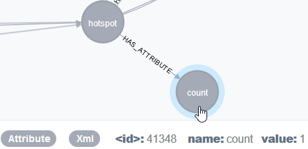
The attribute with the name count contains the number of executions of a SQL statement:
Each element or attribute is also labeled correspondingly with Element or Attribute.
Looking at real data
I want to show you the data from the database in a more nicer way. So, we load our main libraries and initialize the connection to Neo4j database by creating a Graph object (for more details on this have a look at this blog post)
import pandas as pd
from py2neo import Graph

graph = Graph()
We execute a simple query for one XML element and it’s relationships to its attributes.
For example, if we want to display the data of this <hotspot element
<hotspot
    leaf="false"
    value="SELECT id, name FROM types ORDER BY name"
    time="78386"
    count="107">
as graph, we get that information from all the attributes of an element (don’t worry about the syntax of the following two Cypher statements. They are just there to show you the underlying data as an example).
query="""
MATCH (e:Element)-[:HAS_ATTRIBUTE]->(a:Attribute)
WHERE a.value = "SELECT id, name FROM types ORDER BY name"
WITH e as node
MATCH (node)-[:HAS_ATTRIBUTE]->(all:Attribute)
RETURN all.name, all.value
"""
pd.DataFrame(graph.run(query).data())
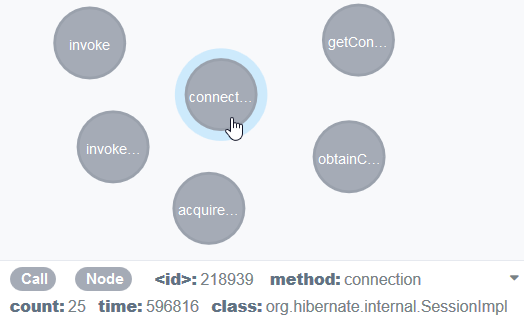
As seen in the picture with the huge graph above, each <hotspot> node refers to the further <node>s, that call the hotspots. In our case, these nodes are the methods in our application that are responsible for the executions of the SQL statements.
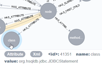
If we list all attributes of such a node, we’ve got plenty of information of the callees of the hotspots. For example these nodes contain information about the method name (method) or the number of executed SQL statements (count):
query="""
MATCH (e:Element)-[:HAS_ATTRIBUTE]->(a:Attribute)
WHERE id(e) = 12 //just select an arbitrary node
RETURN a.name, a.value
"""
pd.DataFrame(graph.run(query).data())
Prepare performance analysis
Because it’s a bit cumbersome to work at the abstraction level of the XML file, let’s enrich this graph with a few better concepts for mining performance problems.
Clean up (optional)
Before executing the first statements, we clean up any preexisting data from previous queries. This is only necessary when you execute this notebook several times on the same data store (like me). It makes the results repeatable and thus more reproducible (a property we should generally strive for!).
query="""
MATCH (n:Node)-[r:CALLS|CREATED_FROM|LEADS_TO]->()
DELETE r, n
RETURN COUNT(r), COUNT(n)"""
graph.run(query).data()
Consolidate the data
We create some new nodes that contain all the information from the XML part of the graph that we need. We simply copy the values of some attributes to new Call nodes.
In our Cypher query, we first retrieve all <node> elements (identified by their “name” property) and some attributes that we need for our analysis. For each relevant information item, we create a variable to retrieve the information later on:
MATCH (n:Element {name: "node"}),
    (n)-[:HAS_ATTRIBUTE]->(classAttribut:Attribute {name : "class"}),
    (n)-[:HAS_ATTRIBUTE]->(methodAttribut:Attribute {name : "methodName"}),
    (n)-[:HAS_ATTRIBUTE]->(countAttribut:Attribute {name : "count"}),
    (n)-[:HAS_ATTRIBUTE]->(timeAttribut:Attribute {name : "time"})
For each <node> element we’ve found, we tag the nodes with the label Node to have a general marker for the JProfiler measurements (which is “node” by coincidence) and mark all nodes that contain information about the calling classes and methods with the label Call:
CREATE
   (x:Node:Call {
We also copy the relevant information from the <node> element’s attributes into the new nodes. We put the value of the class attribute (that consists of the Java package name and the class name) into the fqn (full qualified name) property and add just the name of the class in the class property (just for displaying reasons in the end). The rest is copied as well, including some type conversions for count and time:
        fqn: classAttribut.value,
        class: SPLIT(classAttribut.value,".")[-1],
        method: methodAttribut.value,
        count: toFloat(countAttribut.value),
        time: toFloat(timeAttribut.value)
        })
Additionally, we track the origin of the information by a CREATED_FROM relationship to connect the new nodes later on:
-[r:CREATED_FROM]->(n)
So, the complete query looks like the following and will be executed against the Neo4j data store:
query = """
MATCH (n:Element {name: "node"}),
    (n)-[:HAS_ATTRIBUTE]->(classAttribut:Attribute {name : "class"}),
    (n)-[:HAS_ATTRIBUTE]->(methodAttribut:Attribute {name : "methodName"}),
    (n)-[:HAS_ATTRIBUTE]->(countAttribut:Attribute {name : "count"}),
    (n)-[:HAS_ATTRIBUTE]->(timeAttribut:Attribute {name : "time"})
CREATE
   (x:Node:Call {
        fqn: classAttribut.value,
        class: SPLIT(classAttribut.value,".")[-1],
        method: methodAttribut.value,
        count: toFloat(countAttribut.value),
        time: toFloat(timeAttribut.value)
        })-[r:CREATED_FROM]->(n)
RETURN COUNT(x), COUNT(r)
"""
graph.run(query).data()
We do the same for the <hotspot> elements. Here, the attributes are a little bit different, because we are gathering data from the hotspots that contain information about the executed SQL statements:
query = """
MATCH (n:Element { name: "hotspot"}),
    (n)-[:HAS_ATTRIBUTE]->(valueAttribut:Attribute {name : "value"}),
    (n)-[:HAS_ATTRIBUTE]->(countAttribut:Attribute {name : "count"}),
    (n)-[:HAS_ATTRIBUTE]->(timeAttribut:Attribute {name : "time"})

WHERE n.name = "hotspot"
CREATE
   (x:Node:HotSpot {
        value: valueAttribut.value,
        count: toFloat(countAttribut.value),
        time: toFloat(timeAttribut.value)
        })-[r:CREATED_FROM]->(n)
RETURN COUNT(x), COUNT(r)
"""
graph.run(query).data()
Now, we have many new nodes in our database that are aren’t directly connected. E. g. a Call node looks like this:
So, let’s connect them. How? We’ve saved that information with our CREATED_FROM relationship:
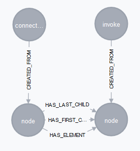
This information can be used to connect the Call nodes as well as the HotSpot nodes.
query="""
MATCH (outerNode:Node)-[:CREATED_FROM]->
      (outerElement:Element)-[:HAS_ELEMENT]->
      (innerElement:Element)<-[:CREATED_FROM]-(innerNode:Node)
CREATE (outerNode)<-[r:CALLS]-(innerNode)
RETURN COUNT(r)
"""
graph.run(query).data()
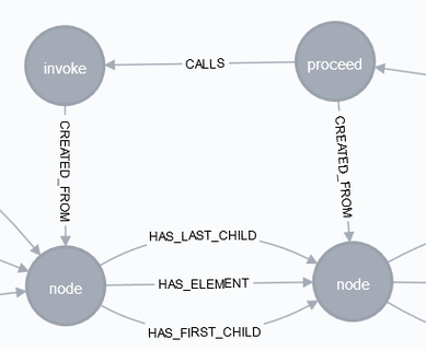
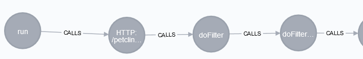
And there we have it! Just click in the Neo4j browser on the relationship CALLS and the you’ll see our call tree from JProfiler as call graph in Neo4j, ready for root cause analysis!
That should be enough for today. So stay tuned for the existing analysis part in the next blog post where we play around with our call graph!
(In case you can’t wait, here is the notebook as draft on GitHub)
Pingback:Mining performance hotspots with JProfiler, jQAssistant, Neo4j and Pandas – Part 2: Root Cause Analysis – feststelltaste