Root Cause Analysis
Conceptual model
All the work before was just there to get a nice graph model that feels more natural. Now comes the analysis part: As mentioned in the introduction, we don’t only want the hotspots that signal that something awkward happened, but also
- the trigger in our application of the hotspot combined with
- the information about the entry point (e. g. where in our application does the problem happen) and
- (optionally) the request that causes the problem (to be able to localize the problem)
Speaking in graph terms, we need some specific nodes of our call tree graph with the following information:
- HotSpot: The executed SQL statement aka the HotSpot node
- Trigger: The executor of the SQL statement in our application aka the Call node with the last class/method call that starts with our application’s package name
- Entry: The first call of our own application code aka the Call node that starts also with our application’s package name
- Request: The Call node with the information about the HTTP request (optional, but because JProfiler delivers this information as well, we use it here in this example)
These points in the call tree should give us enough information that we can determine where to look for improvements in our application.
Challenges
There is one thing that is a little bit tricky to implement: It’s to model what we see as “last” and “first” in Neo4j / Cypher. Because we are using the package name of a class to identify our own application, there are many Call nodes in one call graph part that have that package name. Neo4j would (rightly) return too many results (for us) because it would deliver one result for each match. And a match is also given when a Call node within our application matches the package name. So, how do we mark the first and last nodes of our application code?
Well, take one step at a time. Before we are doing anything awkward, we are trying to store all the information that we know into the graph before executing our analysis. I always favor this approach instead of trying to find a solution with complicated cypher queries, where you’ll probably mix up things easily.
Preparing the query
First, we can identify the request, that triggers the SQL statement, because we configured JProfiler to include that information in our call tree. We simply label them with the label Request.
Identifying all request
query="""
MATCH (x)
WHERE x.fqn = "_jprofiler_annotation_class" AND x.method STARTS WITH "HTTP"
SET x:Request
RETURN COUNT(x)
"""
graph.run(query).data()
Identifying all entry points into the application
Next, we identify the entry points aka first nodes of our application. We can achieve this by first searching all the shortest paths between the already existing Request nodes and all the nodes that have our package name. From all these subgraphs, we take only the single subgraph that has only a single node with the package name of our application. This is the first node that occurs in the call graph when starting from the request (I somehow can feel that there is a more elegant way to do this. If so, please let me know!). We mark that nodes as Entry nodes.
query="""
MATCH
    request_to_entry=shortestPath((request:Request)-[:CALLS*]->(entry:Call))
WHERE
    entry.fqn STARTS WITH "org.springframework.samples.petclinic"
AND
    SINGLE(n IN NODES(request_to_entry)
        WHERE exists(n.fqn) AND n.fqn STARTS WITH "org.springframework.samples.petclinic")
SET
    entry:Entry
RETURN COUNT(entry)
"""
graph.run(query).data()
With the same approach, we can mark all the calls that trigger the execution of the SQL statements with the label Trigger.
query="""
MATCH
    trigger_to_hotspot=shortestPath((trigger:Call)-[:CALLS*]->(hotspot:HotSpot))
WHERE
    trigger.fqn STARTS WITH "org.springframework.samples.petclinic"
AND
    SINGLE(n IN NODES(trigger_to_hotspot)
        WHERE exists(n.fqn) AND n.fqn STARTS WITH "org.springframework.samples.petclinic")
SET
    trigger:Trigger
RETURN count(trigger)
"""
graph.run(query).data()
After marking all the relevant nodes, we connect them via a new relationshop LEADS_TO to enable more elegant queries later on.
query="""
MATCH
   (request:Request)-[:CALLS*]->
       (entry:Entry)-[:CALLS*]->
           (trigger:Trigger)-[:CALLS*]->
               (hotspot:HotSpot)
CREATE UNIQUE
    (request)-[leads1:LEADS_TO]->
        (entry)-[leads2:LEADS_TO]->
            (trigger)-[leads3:LEADS_TO]->(hotspot)
RETURN count(leads1), count(leads2), count(leads3)
"""
graph.run(query).data()
Getting results
All the previous steps where needed to enable this simple query, that gives us the spots in the application, that lead eventually to the hotspots!
query="""
MATCH
   (request:Request)-[:LEADS_TO]->
       (entry:Entry)-[:LEADS_TO]->
           (trigger:Trigger)-[:LEADS_TO]->
               (hotspot:HotSpot)
RETURN
    request.method as request,
    request.count as sql_count,
    entry.class as entry_class,
    entry.method as entry_method,
    trigger.class as trigger_class,
    trigger.method as trigger_method,
    hotspot.value as sql,
    hotspot.count as sql_count_sum
"""
hotspots = pd.DataFrame(graph.run(query).data())
hotspots.head()
The returned data consists of
- request: the name of the HTTP request
- sql_count: the number of SQL statements caused by this HTTP request
- entry_class: the class name of the entry point into our application
- entry_method: the method name of the entry point into our application
- trigger_class: the class name of the exit point out of our application
- trigger_method: the method name of the exit point out of our application
- sql: the executed SQL statement
- sql_count_sum: the amount of all executed SQL statements of the same kind
A look at a subgraph
If we take a look at the Neo4j browser and execute the statement from above but returning the nodes, aka
MATCH
   (request:Request)-[:LEADS_TO]->
       (entry:Entry)-[:LEADS_TO]->
           (trigger:Trigger)-[:LEADS_TO]->
               (hotspot:HotSpot)
RETURN
    request, entry, trigger, hotspot
we get a nice overview of all our performance hotspots, e. g.
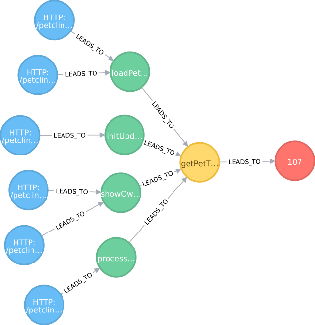
With this graphical view, it’s easy to see the connection between the requests, our application code and the hotspots.
Albeit this view is nice for exploration, it’s not actionable. So let’s use Pandas to shape the data to knowledge!
In-depth analysis
First, we have a look which parts in the application trigger all the SQLs. We simply group some columns to get a more dense overview:
sqls_per_method = hotspots.groupby([
    'request',
    'entry_class',
    'entry_method',
    'trigger_class',
    'trigger_method']).agg(
        {'sql_count' : 'sum',
         'request' : 'count'})
sqls_per_method
We see immediately that we have an issue with the loading of the pet’s owners via the OwnerController. Let’s look at the problem from another perspective: What kind of data is loaded by whom from the tables. We simply chop the SQL and extract just the name of the database table (in fact, the regex is so simple that some of the tables weren’t identified. But because these are special cases, we can ignore them):
hotspots['table'] = hotspots['sql'].\
    str.upper().str.extract(
        r".*(FROM|INTO|UPDATE) ([\w\.]*)",
        expand=True)[1]
hotspots['table'].value_counts()
And group the hotspots accordingly.
grouped_by_entry_class_and_table = hotspots.groupby(['entry_class', 'table'])[['sql_count']].sum()
grouped_by_entry_class_and_table
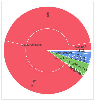
Now we made the problem more obvious: The class OwnerController works heavily with the PETS table and the pet’s TYPES table. Surely an error in our program.
Let’s visualize the problem with a nice donut chart in Bokeh:
from bokeh.charts import Donut, show, output_notebook

plot_data = grouped_by_entry_class_and_table.reset_index()
d = Donut(plot_data, label=['entry_class', 'table'],
          values='sql_count',
          text_font_size='8pt',
          hover_text='sql_count'
         )
output_notebook()
show(d)
You could also have a look at the most problematic spot in the application by grouping the data by the class and the method that triggers the execution of the most SQL statements.
hotspots.groupby(['trigger_class', 'trigger_method'])[['sql_count']].sum().sort_values(
    by='sql_count', ascending=False).head(5)
Again, the JdbcOwnerRepositoryImpl is heavily working with other data.
This gives you a very actionable information where you can start improving!
Result
The overall result of this analysis is clearly an application problem and a sign of the famous N+1 query problem that’s almost typical for any application that uses a database without care.
If you look at the corresponding source code, you’ll find spots in your application like the one below in the JdbcOwnerRepositoryImpl class:
public void loadPetsAndVisits(final Owner owner) {
        Map<String, Object> params = new HashMap<>();
        params.put("id", owner.getId());

        final List<JdbcPet> pets = this.namedParameterJdbcTemplate.query(
            "SELECT pets.id, name, birth_date, type_id, owner_id,
             visits.id as visit_id, visit_date, description, pet_id
             FROM pets LEFT OUTER JOIN visits ON  pets.id = pet_id
             WHERE owner_id=:id", params, new JdbcPetVisitExtractor());

        Collection<PetType> petTypes = getPetTypes();
        for (JdbcPet pet : pets) {
            pet.setType(EntityUtils.getById(petTypes, PetType.class, pet.getTypeId()));
            owner.addPet(pet);
        }
    }
E. g. we see data that isn’t needed in the UI, but loaded from a database within a loop. This can surely be improved!
Discussion and Limitations
This approach for mining performance problem follows a simple pattern:
- Load all the data you need into Neo4j
- Encode your problems/concepts in Cypher
- Retrieve the data for further analysis in Pandas
With these steps, you quickly drill down to the root cause of problems.
But there are also limitations:
- There is one big problem with this approach if you use want to export big hotspot call trees in JProfiler. It simply doesn’t work when the XML data is getting too big (> 500 MB)
- One approach would be the get direct access to the HotSpot data in JProfiler. I still have to ask the developers of JProfiler if this would be possible.
- The other approach that we’re trying to do at work is to export just the Call Tree (because it’s not so much data) as a XML file, import it into Neo4j (by using jQAssistant, too) and calculate the HotSpots ourself.
- Additionally, jQAssistant isn’t able to load huge (> 2 GB) XML files out of the box, but there may be some tweaks to get that working, too.
- Identifying your own application just by the package name makes the Cypher queries a lot more complex. If you can (and if you have something that’s called an architecture), it should be easier for you to just use class names to determine the entry points into your application (the same goes for determining the triggers).
Overall, I’m really happy with this approach because it immediately shows me the performance pain points in our application.
Summary
I hope that you take away many new ideas for your analysis of software data:
- It’s easy to export graph like performance measures from JProfiler
- You can read XML content with jQAssistant
- With coding your knowledge into a graph step by step, you can easily achieve almost anything with Neo4j
- Post-processing good data with Pandas and Bokeh is easy like pie!
The main idea was to load a huge graph with all the information and reduce it to just the specific information we need for action. In general, I use this approach to mine my way through any graph-based data format like XML files or other software structures.
Last but not least: Many thanks to my student Andreas, who had to prototype some of my crazy graph query ideas 🙂
And as always: I’ll be happy to answer your questions and please let me know what you think about this approach!
Pingback:Mining performance hotspots with JProfiler, jQAssistant, Neo4j and Pandas – Part 1: The Call Graph – feststelltaste