Introduction
In his book Software Design X-Rays, Adam Tornhill shows a nice metric to find out if some parts of your code are coupled regarding their conjoint changes: Temporal Coupling.
In this and the next blog posts, I’m playing around with Adam’s ideas (and more) to find hidden dependencies of code parts based on version control data.
In this part, we just want to spot co-changing files which are files that change within the same commit.
As almost always, we are using Python and pandas for this analysis.
Data
With the help of a little helper library, we extract relevant log data from a Git repository. In this case, we are just using a synthetic repository to easier check that everything is working as expected.
Here are all files and all the commits from the repository:
from lib.ozapfdis.git_tc import log_numstat
commits = log_numstat("../../synthetic_repo//")
commits
We see that some files change often together (like “a” and “b” or “b” and “d”) and some files are completely changing alone (like “e”).
Let’s get rid of all the unneeded columns first by just the columns that we really need for this analysis.
commits = commits[['file', 'sha']]
commits.head()
Idea
In this analysis, we need to create a relationship from each changed file to all changed file within the same commit.
I tried different things there with various data transformations, but in the end, the following stupid straightforward approach worked best: We just assign to each file in a commit all files of the same commit and count the occurrence of these relationships.
This gives us the perspectives on co-working changes that we want.
Analysis
To implement the idea of above, we can use the pd.merge command of pandas to combine the commits DataFrame with itself. The key here is to use an outer join to expand each file in a commit (designated by the value sha) to all the files of a commit (again, designated by the values in sha).
import pandas as pd

commit_counts = pd.merge(
    commits,
    commits,
    left_on='sha',
    right_on='sha',
    suffixes=['','_other'],
    how='outer')
commit_counts.head()
With this, e. g. the last commit (= first entries in the DataFrame) was expanded from
0   b   a2abe69
1   d   a2abe69
to
0   b   a2abe69     b
1   b   a2abe69     d
2   d   a2abe69     b
3   d   a2abe69     d
with the additional column of all files of the commit.
Because we’re only interested of co-changing files, we can filter out all entries for file changes of the same file.
commit_counts = commit_counts[commit_counts['file'] != commit_counts['file_other']]
commit_counts.head()
We then can count the same commit relationships with the groupby command.
commit_coupling = commit_counts.groupby(['file', 'file_other']).count()
commit_coupling.head()
For also want to know the amount of all changes for each file to get the degree of the overall coupling between co-changing files. For this, we can use the groupby command on the file index column together with the transform method to calculate the number of changes per file.
commit_coupling['all_changes'] = commit_coupling.groupby(['file']).sha.transform('sum')
commit_coupling.head()
We further calculate the ratio between each changed file to the number of all changes for all files per commit. A high ratio gives us an indicator for pairwise files that change together very often.
commit_coupling['ratio'] = commit_coupling['sha'] / commit_coupling['all_changes']
commit_coupling
At last step, we do some housekeeping of the data to get a nicely sorted list of co-changing files.
coupling_list = commit_coupling.reset_index().sort_values(
    by=['ratio', 'file'], ascending=False)
coupling_list.rename(columns={"sha" : "co-changing"})
coupling_list = coupling_list.rename(columns={"sha" : "co-changing"})
coupling_list = coupling_list.reset_index(drop=True)
coupling_list
With this result, we can e.g. see in the first three rows that the files “d”,”c” and “a” always change with the file “b”.
In detail, you can read and interpret the table like this:
- Row with index
0: For all changes of “d”, “b” was always changed. This shows a high change dependency from the file “d” to the file “b”. In other words: If one changes “d”, something has to be changed in “b”, too. - Row with index
3: If “b” was changed, “a” was changed in 4 out of 7 cases (=commits) as well. Together with the row indexed2, we can see that “a” changes always with “b”, but “b” doesn’t always change with “a”. - Row with index
5: If “b” was changed, “c” was changed in one case. This shows a slight (or even negligible) dependency from “b” to “c” (and maybe even “c” to “b”, because only one commit could also be coincident).
If you are more into graphs, here are all the change relationships between the files with their ratio measure:
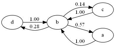
Note: The file “e” isn’t occurring in the table because it’s getting changed completely independent.
Visualizations
We can also try to draw a diagram that suits the tiny amount of data that we have. In our case, we use a D3 chord diagram to explore the coupling of co-changing files interactively. Pandas can output the data in a JSON format needed by the used D3 visualization.
coupling_list[['file','file_other','co-changing']].to_json(
    "chord_coupling_data.json", orient='values')
The chord diagram gives us hint about the inherent coupling of files based on co-changing.
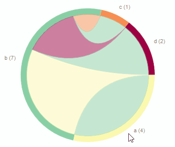
You can find the interactive version of this visualization here.
Summary
We’ve seen that we can spot co-changing files with the help of pandas straightforward.
Doing it step by step allows us also to step-wise refine the analysis to our own circumstances. For example, we could define co-changing files as files that not only change within a commit, but on the same day. We could also find peaks of co-changing actions that could lead us to chaotic changes in code.
But for now, we leave it there.
You can find the notebook on GitHub.
Pingback:Checking the modularization of software systems by analyzing co-changing source code files – feststelltaste