Introduction
In this short blog post, I want to show you an idea where you take some very detailed datasets from a software project and transform it into a representation where management can reason about. For this,
- we take the utilization of a web application measured by the code coverage during user interactions
- we estimate the investments in the software by the number of changes
- we aggregate the data to something management can understand
- we visualize the results in a SWOT (Strengths, Weaknesses, Opportunities, Threats) matrix
This little picture summarizes the main ideas where the data comes from:
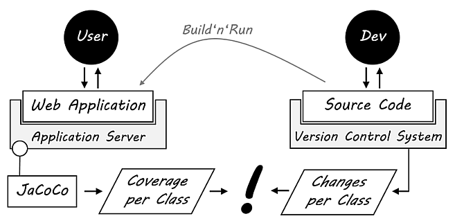
Let’s get some insights!
Utilization of a production system
As proxy for utilization, we take the code coverage of a web application during the live operation with user interactions. I’ve collected that data by attaching the JaCoCo agent to the Java process (for details on how to do that see my blog post “Visualizing Production Coverage with JaCoCo, Pandas and D3”).
The result is a dataset with covered lines (= run through lines of code) per class. We read that into a Pandas DataFrame.
import pandas as pd

coverage = pd.read_csv("datasets/jacoco_production_coverage_spring_petclinic.csv")
coverage.head()
We need to calculate some additional variables for our analysis later on: The lines of code per class and the ratio of the covered lines of code to all lines of code per class.
coverage['lines'] = coverage.LINE_MISSED + coverage.LINE_COVERED
coverage['covered'] = coverage.LINE_COVERED / coverage.lines
coverage.head()
Next, we create a unique identifier for connecting the coverage data to the number of changes per class. We choose the fully qualified name (“fqn”) of a class as key for this, set this variable as an index and only take the columns that we need later.
coverage['fqn'] = coverage.PACKAGE + "." + coverage.CLASS
coverage_per_class = coverage.set_index('fqn')[['lines', 'covered']]
coverage_per_class.head()
Investments in code
As a proxy for the investments we took into our software, we choose the number of changes per file. For this, we need a log of our version control system. With Git, a simple numstat log does the job. We can get a list for each change of a file including the added and deleted lines with the command
git log --no-merges --no-renames --numstat --pretty=format:""We kind of hacked the git log pretty format option, but it does the job. We read that dataset into a DataFrame as well, using the tabular as a separator and specifying some column names manually.
changes = pd.read_csv(
    "datasets/git_log_numstat_spring_petclinic.log",
    sep="\t",
    names=['additions', 'deletions', 'path'])
changes.head()
As with the coverage data, we need a unique identifier per class. We can create that based on the path of each file.
changes['fqn'] = changes.path.str.extract(
    "/java/(.*)\.java",
    expand=True)[0]
changes['fqn'] = changes.fqn.str.replace("/", ".")
changes['fqn'][0]
Different to the coverage dataset, we have multiple entries per file (for each change of that file). We need to group the changes by the fqn of each file or class respectively. We just take the path column that holds the number of changes for each class and renames that column to changes. The result is a Series of the number of changes per file.
changes_per_file = changes.groupby('fqn').path.count()
changes_per_file.name = "changes"
changes_per_file.head()
Joining of the datasets
Next, we can join the two different datasets with the DataFrames’ join method.
analysis = coverage_per_class.join(changes_per_file)
analysis.head()
Creating a higher technical view
OK, now to the key idea of this analysis. We need to raise the very fine-granular data on class level to a more higher-level where we can reason about in a better way. For this, we derive higher-level perspectives based on the fqn of the classes. For technical components, we can do this in our case based on the package name because the last part of the package name contains the name of the technical component.
analysis['tech'] = analysis.index.str.split(".").str[-2]
analysis.head()
We can now aggregate our fine-granular data to a higher-level representation by grouping the data accordingly to the technical components. For the agg function, we provide a dictionary with the aggregation methods for each column.
tech_insights = analysis.groupby('tech').agg({
    "lines" : "sum",
    "covered": "mean",
    "changes" : "sum"
    })
tech_insights.head()
With the help of a (self-written) little visualization, we can now create a SWOT matrix from our data.
%matplotlib inline
from lib.ausi import portfolio
portfolio.plot_diagram(tech_insights, "changes", "covered", "lines");

Discussion
- In the lower right, we can see that we changed the
jdbccomponent very often (aka invested much money) but the component isn’t used at all. A clear failure of investments (OK, in this case, it’s an alternative implementation of the database access, but we could also delete this code completely without any side effects). - Above, we see that we also invested heavily in the
webcomponent, but this isn’t used as much as it should be (in relation to the changes). Maybe we can find code in this component that isn’t needed anymore. - The
petclinic(a base component),service,jpaandmodelcomponents in the upper left are used very often with low changes (aka investments). This is good!
Creating a domain view
Next, we want to create a view that non-technical people can understand. For this, we use the naming schema of the classes to identify which business domain each class belongs to.
analysis['domain'] = "Other"

domains = ["Owner", "Pet", "Visit", "Vet", "Specialty", "Clinic"]
for domain in domains:
    analysis.loc[analysis.index.str.contains(domain), 'domain'] = domain

analysis.head()
Like with the technical components, we group the business aspects accordingly but also translate the technical terms into non-technical ones.
domain_insights = analysis.groupby('domain').agg({
    "lines" : "sum",
    "covered": "mean",
    "changes" : "sum"
    })
domain_insights = domain_insights.rename(columns=
   {"lines": "Size", "covered" : "Utilization", "changes" : "Investment"})
domain_insights.head()
Again, we plot a SWOT matrix with the data in the DataFrame.
portfolio.plot_diagram(domain_insights, "Investment", "Utilization", "Size");

Discussion
- The investments into the classes around
Clinicin the upper left of the matrix were worthwhile. - We have to have a look at the trend of
PetandOwnerrelated classes because albeit we’ve invested heavily in this parts, they aren’t used so much. - For the
VisitandVetcomponents in the lower right, we should take a look at if those components are worthwhile further improvements or candidates for removal. - The
Othercomponent has good chances to be improved the right way in the near future by only developing the parts further that are really needed.
Conclusion
OK, we’ve seen how we can take some very fine-granular dataset, combine them and bring them to a higher-level perspective. We’ve also visualized the results of our analysis with a SWOT matrix to quickly spot parts of our software system that are good or bad investments.
What do you think about this approach? Do you like the idea? Or is this complete nonsense? Please leave me a comment!
Your can find the original Jupyter notebook on GitHub.
Update 25.04.2018: Fixed bug with interchanged axes in last plot.
Pingback:My talk at JAX 2018 – feststelltaste
Pingback:Data Analysis in Software Development – feststelltaste